Note
This is example is available as a Jupyter notebook. Download it and all
necessary data files here.
L1 Norm Regression
This example implements a regression model which minimizes mean absolute error as a fitting criteria. This metric cannot be handled by the typical Ordinary Least Squares (OLS) regression implementation, but is well suited to linear programming (and therefore, to Gurobi!).
L1 norm regressionaims to choose weights \(w\) in order to minimize the following loss function:
To model the L1 regression loss function using linear programming, we need to introduce a number of auxiliary variables. Here \(I\) is the set of data points and \(J\) the set of fields. Response values \(y_i\) are predicted from predictor values \(x_{ij}\) by fitting coefficients \(w_j\). To handle the absolute value, non-negative continuous variables \(u_i\) and \(v_i\) are introduced.
We start with the usual imports for gurobipy-pandas models. Additionally, we import some sklearn modules, both to load an example dataset and to help perform model validation.
[1]:
import gurobipy as gp
from gurobipy import GRB
import gurobipy_pandas as gppd
import pandas as pd

from sklearn import datasets
from sklearn.preprocessing import StandardScaler
from sklearn.model_selection import train_test_split
We first load the diabetes regression dataset into pandas dataframes, then perform scaling and a train-test split. Additionally, we add a constant column to capture an intercept term.
[3]:
diabetes_X, diabetes_y = datasets.load_diabetes(return_X_y=True, as_frame=True)
scaler = StandardScaler()
diabetes_X_scaled = pd.DataFrame(
    data=scaler.fit_transform(diabetes_X),
    columns=diabetes_X.columns,
    index=diabetes_X.index,
)
diabetes_X_scaled["const"] = 1.0
X_train, X_test, y_train, y_test = train_test_split(
    diabetes_X_scaled, diabetes_y, random_state=42
)
X_train
[3]:
| age | sex | bmi | bp | s1 | s2 | s3 | s4 | s5 | s6 | const | |
|---|---|---|---|---|---|---|---|---|---|---|---|
| 16 | -0.115937 | -0.938537 | 0.889214 | 1.038895 | 0.516642 | -0.501640 | 1.564414 | -0.830301 | 1.099061 | 0.586922 | 1.0 |
| 408 | 1.335088 | -0.938537 | -1.059520 | 2.269385 | 0.661281 | 0.406893 | -0.370637 | 0.496320 | 1.220180 | 0.848171 | 1.0 |
| 432 | 0.189542 | -0.938537 | 1.161130 | -0.119214 | 1.210908 | 0.940162 | -0.061029 | 0.488562 | 1.170736 | 2.241496 | 1.0 |
| 316 | 0.342282 | 1.065488 | 0.300062 | 0.025550 | 0.024870 | -0.448971 | -0.680245 | 0.721302 | 1.576064 | 0.848171 | 1.0 |
| 3 | -1.872441 | -0.938537 | -0.243771 | -0.770650 | 0.256292 | 0.525397 | -0.757647 | 0.721302 | 0.476983 | -0.196823 | 1.0 |
| ... | ... | ... | ... | ... | ... | ... | ... | ... | ... | ... | ... |
| 106 | -2.025181 | -0.938537 | -1.603353 | -0.915414 | -0.958674 | -0.732065 | 0.171178 | -0.830301 | -1.250310 | -1.764314 | 1.0 |
| 270 | 0.113172 | 1.065488 | 0.639957 | 1.762713 | -0.785107 | -0.995407 | 0.325982 | -0.830301 | 0.181658 | 0.325674 | 1.0 |
| 348 | 0.647761 | -0.938537 | -0.425049 | -0.119214 | -0.090841 | -0.620144 | 1.641816 | -0.830301 | -0.229228 | -0.022657 | 1.0 |
| 435 | -0.268676 | -0.938537 | -0.493028 | -0.843032 | -0.351191 | 0.097465 | -0.370637 | -0.054499 | -0.808569 | -0.806403 | 1.0 |
| 102 | -1.948811 | -0.938537 | 0.594638 | -0.336359 | 0.776992 | 0.525397 | 1.177404 | -0.830301 | -0.108108 | -0.022657 | 1.0 |
331 rows × 11 columns
Model Formulation
Create the Gurobi model:
[4]:
model = gp.Model()
Then we create an unbounded variable for each column coefficient. Here we use the free function gppd.add_vars to create these variables. Note that what we want here is one variable per column, and in pandas, the column labels are also an index. So, we can pass this index directly to the gurobipy-pandas function to create a Series of variables aligned to this column index.
[5]:
coeffs = gppd.add_vars(model, X_train.columns, name="coeff", lb=-GRB.INFINITY)
model.update()
coeffs
[5]:
age        <gurobi.Var coeff[age]>
sex        <gurobi.Var coeff[sex]>
bmi        <gurobi.Var coeff[bmi]>
bp          <gurobi.Var coeff[bp]>
s1          <gurobi.Var coeff[s1]>
s2          <gurobi.Var coeff[s2]>
s3          <gurobi.Var coeff[s3]>
s4          <gurobi.Var coeff[s4]>
s5          <gurobi.Var coeff[s5]>
s6          <gurobi.Var coeff[s6]>
const    <gurobi.Var coeff[const]>
Name: coeff, dtype: object
Given this column-oriented series and our training dataset, we can formulate the linear relationships representing the regression formula using native pandas operations:
[6]:
relation = (X_train * coeffs).sum(axis="columns")
relation
[6]:
16     -0.11593687913484965 coeff[age] + -0.938536660...
408    1.3350883235096624 coeff[age] + -0.93853666088...
432    0.1895421108955739 coeff[age] + -0.93853666088...
316    0.34228160591078566 coeff[age] + 1.06548847975...
3      -1.8724410718097853 coeff[age] + -0.9385366608...
                             ...
106    -2.025180566824997 coeff[age] + -0.93853666088...
270    0.11317236338796802 coeff[age] + 1.06548847975...
348    0.6477605959412093 coeff[age] + -0.93853666088...
435    -0.26867637415006146 coeff[age] + -0.938536660...
102    -1.9488108193173912 coeff[age] + -0.9385366608...
Length: 331, dtype: object
To incorporate the absolute error component, we need to introduce the variables \(u_i\) and \(v_i\), and constrain them such that they measure the error for each data point. This can be done compactly using the gppd dataframe accessor and method chaining:
[7]:
fit = (
    relation.to_frame(name="MX")
    .gppd.add_vars(model, name="u")
    .gppd.add_vars(model, name="v")
    .join(y_train)
    .gppd.add_constrs(model, "target == MX + u - v", name="fit")
)
model.update()
fit
[7]:
| MX | u | v | target | fit | |
|---|---|---|---|---|---|
| 16 | -0.11593687913484965 coeff[age] + -0.938536660... | <gurobi.Var u[16]> | <gurobi.Var v[16]> | 166.0 | <gurobi.Constr fit[16]> |
| 408 | 1.3350883235096624 coeff[age] + -0.93853666088... | <gurobi.Var u[408]> | <gurobi.Var v[408]> | 189.0 | <gurobi.Constr fit[408]> |
| 432 | 0.1895421108955739 coeff[age] + -0.93853666088... | <gurobi.Var u[432]> | <gurobi.Var v[432]> | 173.0 | <gurobi.Constr fit[432]> |
| 316 | 0.34228160591078566 coeff[age] + 1.06548847975... | <gurobi.Var u[316]> | <gurobi.Var v[316]> | 220.0 | <gurobi.Constr fit[316]> |
| 3 | -1.8724410718097853 coeff[age] + -0.9385366608... | <gurobi.Var u[3]> | <gurobi.Var v[3]> | 206.0 | <gurobi.Constr fit[3]> |
| ... | ... | ... | ... | ... | ... |
| 106 | -2.025180566824997 coeff[age] + -0.93853666088... | <gurobi.Var u[106]> | <gurobi.Var v[106]> | 134.0 | <gurobi.Constr fit[106]> |
| 270 | 0.11317236338796802 coeff[age] + 1.06548847975... | <gurobi.Var u[270]> | <gurobi.Var v[270]> | 202.0 | <gurobi.Constr fit[270]> |
| 348 | 0.6477605959412093 coeff[age] + -0.93853666088... | <gurobi.Var u[348]> | <gurobi.Var v[348]> | 148.0 | <gurobi.Constr fit[348]> |
| 435 | -0.26867637415006146 coeff[age] + -0.938536660... | <gurobi.Var u[435]> | <gurobi.Var v[435]> | 64.0 | <gurobi.Constr fit[435]> |
| 102 | -1.9488108193173912 coeff[age] + -0.9385366608... | <gurobi.Var u[102]> | <gurobi.Var v[102]> | 302.0 | <gurobi.Constr fit[102]> |
331 rows × 5 columns
Each step of the above code appends a new column to the returned dataframe:
Start with the column “MX”, representing the \(Xw\) term
Append a column of new variables \(u_i\) (one for each data point)
Append a column of new variables \(v_i\) (one for each data point)
Join the true target data from
y_trainAdd one constraint per row such that
u_i - v_imeasures the error between prediction and target
Now we are in a position to formulate the mean absolute error expression, and minimize it in the objective function:
[8]:
abs_error = fit["u"] + fit["v"]
mean_abs_error = abs_error.sum() / fit.shape[0]
model.setObjective(mean_abs_error, sense=GRB.MINIMIZE)
Extracting Solutions
With the model formulated, we solve it using the Gurobi Optimizer:
[9]:
model.optimize()
Gurobi Optimizer version 12.0.1 build v12.0.1rc0 (linux64 - "Ubuntu 22.04.3 LTS")

CPU model: Intel(R) Xeon(R) Platinum 8375C CPU @ 2.90GHz, instruction set [SSE2|AVX|AVX2|AVX512]
Thread count: 1 physical cores, 2 logical processors, using up to 2 threads

Optimize a model with 331 rows, 673 columns and 4303 nonzeros
Model fingerprint: 0x2dc542aa
Coefficient statistics:
  Matrix range     [1e-03, 4e+00]
  Objective range  [3e-03, 3e-03]
  Bounds range     [0e+00, 0e+00]
  RHS range        [2e+01, 3e+02]
Presolve time: 0.01s
Presolved: 331 rows, 673 columns, 4303 nonzeros

Iteration    Objective       Primal Inf.    Dual Inf.      Time
       0      handle free variables                          0s
     364    4.3725902e+01   0.000000e+00   0.000000e+00      0s

Solved in 364 iterations and 0.02 seconds (0.02 work units)
Optimal objective  4.372590220e+01
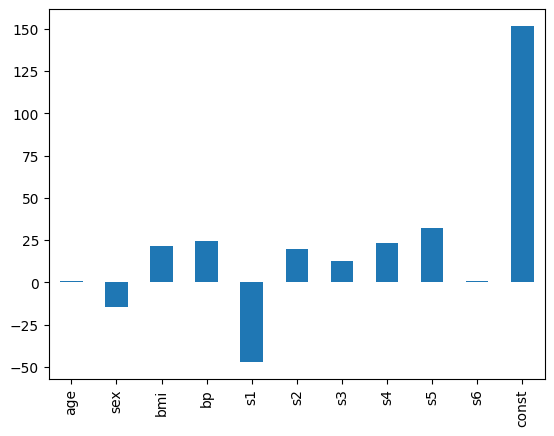
Using the series accessor, we can extract the result coefficients as a series and display them on a plot:
[10]:
coeffs.gppd.X.plot.bar()
Matplotlib is building the font cache; this may take a moment.
[10]:
<Axes: >

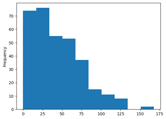
We can also extract the distribution of errors from the abs_error series we constructed, and plot the results as a histogram:
[11]:
# abs_error is a Series of linear expressions
abs_error.head()
[11]:
16       u[16] + v[16]
408    u[408] + v[408]
432    u[432] + v[432]
316    u[316] + v[316]
3          u[3] + v[3]
dtype: object
[12]:
# .gppd.get_value() evaluates these expressions at the current solution
abs_error.gppd.get_value().plot.hist();
